e2tree turns the ensemble's internal structure into a pairwise dissimilarity matrix, then uses that matrix to grow a single decision tree. This page covers the math behind each step.
A tree-based ensemble of B trees assigns every observation to a terminal node in each tree. Two observations that frequently share a terminal node are, in the ensemble's view, similar. This intuition is formalised as the co-occurrence matrix O.
Each entry is a weighted co-occurrence measure. The numerator accumulates the node goodness-of-fit Wtij|b each time observations i and j share a leaf; the denominator normalises by the larger of the two marginal sums:
The corresponding dissimilarity matrix is:
For classification, Wtij|b = Rt is the correct classification rate of the node where i and j meet in tree b (proportion of correctly classified training observations in that node). D is symmetric, non-negative, with zero diagonal, and values in [0, 1]. Computed by createDisMatrix(), with optional parallelisation.
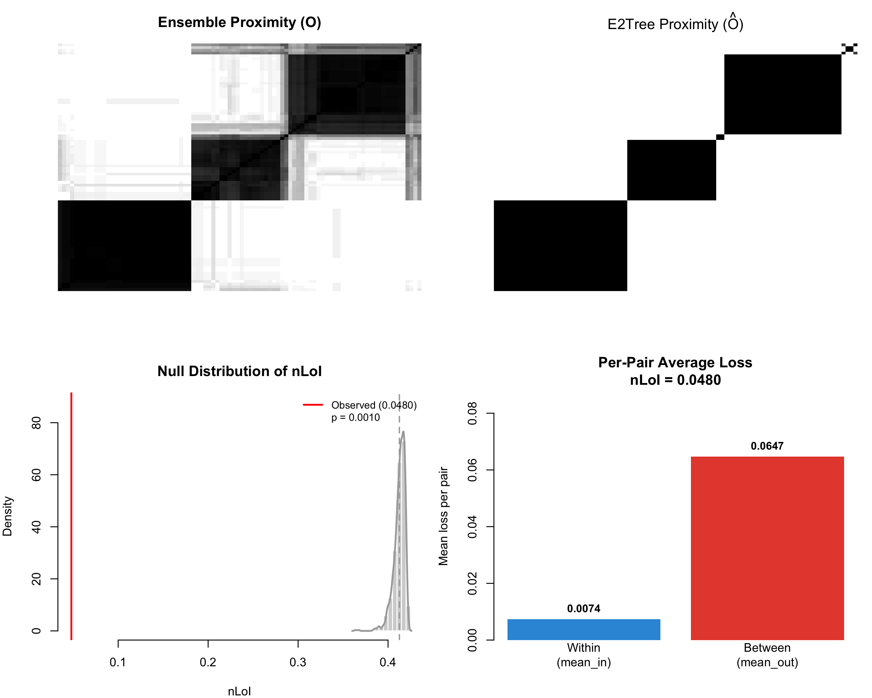
eValidation(). Warmer cells indicate higher co-occurrence frequency (lower dissimilarity); the block structure reflects the underlying class separation learned by the ensemble.
e2tree() constructs the tree recursively. At each node the algorithm searches for the binary split — over all predictors and candidate thresholds — that maximises the reduction in within-group weighted dissimilarity:
Impurity at a node is the average intra-group dissimilarity. Splitting continues until any stopping rule is triggered:
impTotal — minimum node impurity to attempt a splitmaxDec — minimum impurity decrease requiredn — minimum observations in a nodelevel — maximum tree depthIn the classification setting, the response variable is a factor. e2tree computes the dissimilarity matrix from the ensemble's proximity (co-occurrence in terminal nodes), then fits a tree whose leaf predictions are the majority class within each node.
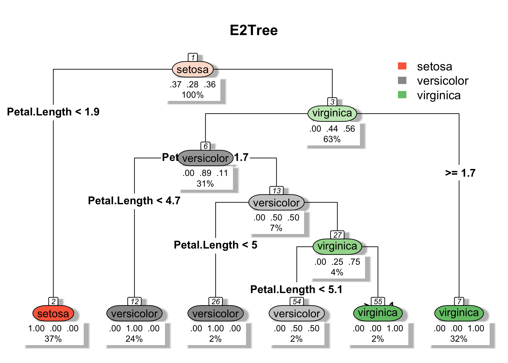
Terminal node purity — the proportion of observations belonging to the predicted class — provides a local measure of classification confidence. The tree produces decision rules domain experts can read directly.
Leaf node prediction for a new observation follows the standard CART convention: route the observation through the split rules to a terminal node; the prediction is the majority class of the training observations in that node, weighted by the ensemble's dissimilarity structure.
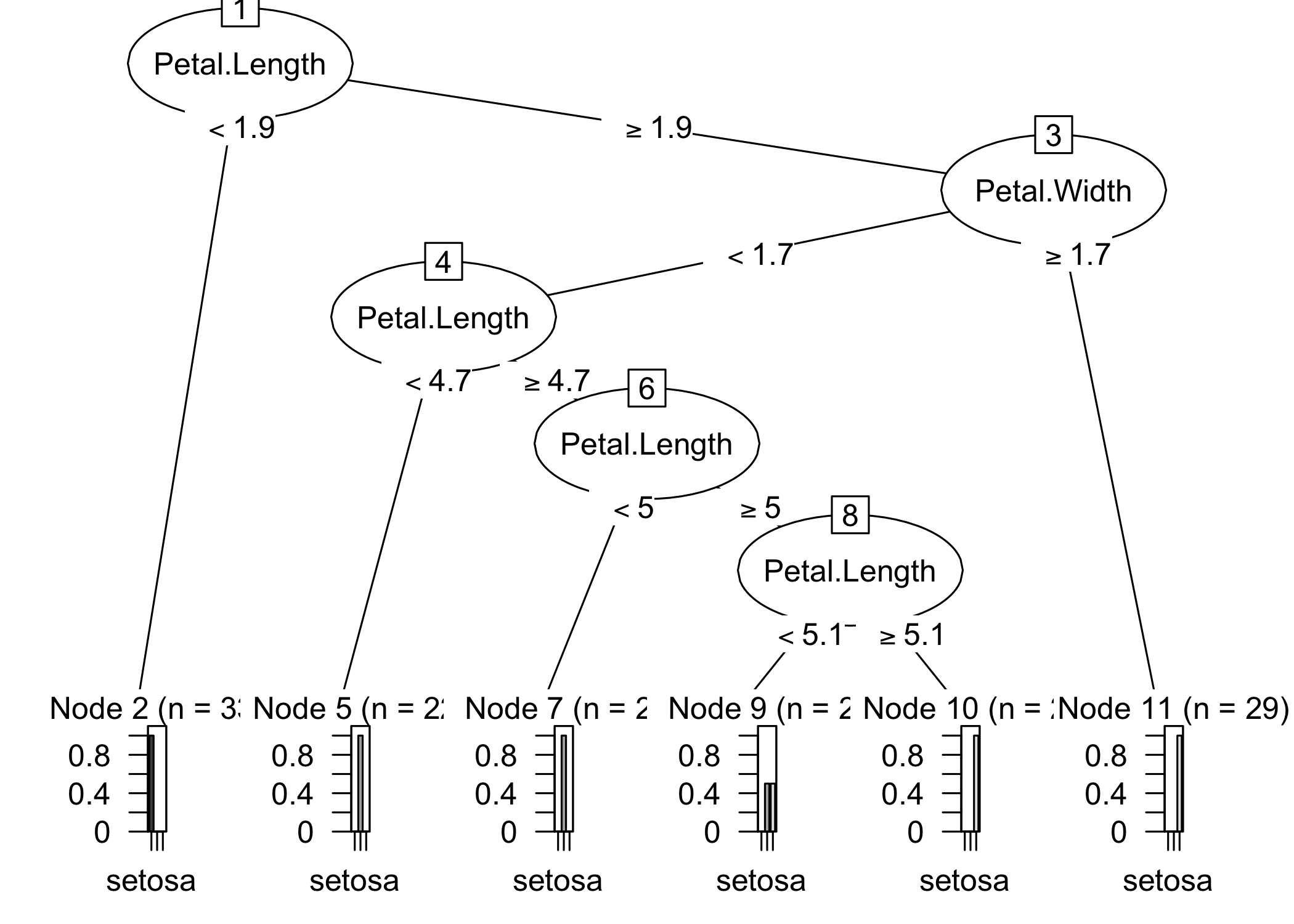
Three-class problem on 150 observations. e2tree recovers perfect setosa separation and near-perfect discrimination between versicolor and virginica in 6 terminal nodes — with 2 split variables.
Included in the package as data(credit). Demonstrates e2tree on an imbalanced binary classification task typical in real-world finance and risk modelling.
Extending e2tree to regression required redefining the goodness-of-fit weight W. The co-occurrence formula has the same structure as the classification case, but the weight now uses the normalised mean squared error (NMSE) at the node: nodes where the ensemble predicts poorly contribute less to the co-occurrence of their observations.
Formally, the regression weight is defined as:
where , p(t) = n(t)/N is the proportion of observations in node t, and MSEmax is the theoretical maximum MSE under the Jacobson bound. Two observations sharing a leaf only count toward co-occurrence to the extent that the ensemble predicts accurately in that node.
The extension is fully described in the 2026 paper in Applied Stochastic Models in Business and Industry. The R implementation follows the same workflow as the classification case.
eValidation() measures how closely the e2tree's proximity structure matches the original ensemble's. It computes concordance between O and the tree's own proximity matrix, returning a numeric score and a heatmap.
measures() — quantitative concordance metricsproximity() — tree proximity heatmapplot() — visualise fidelity
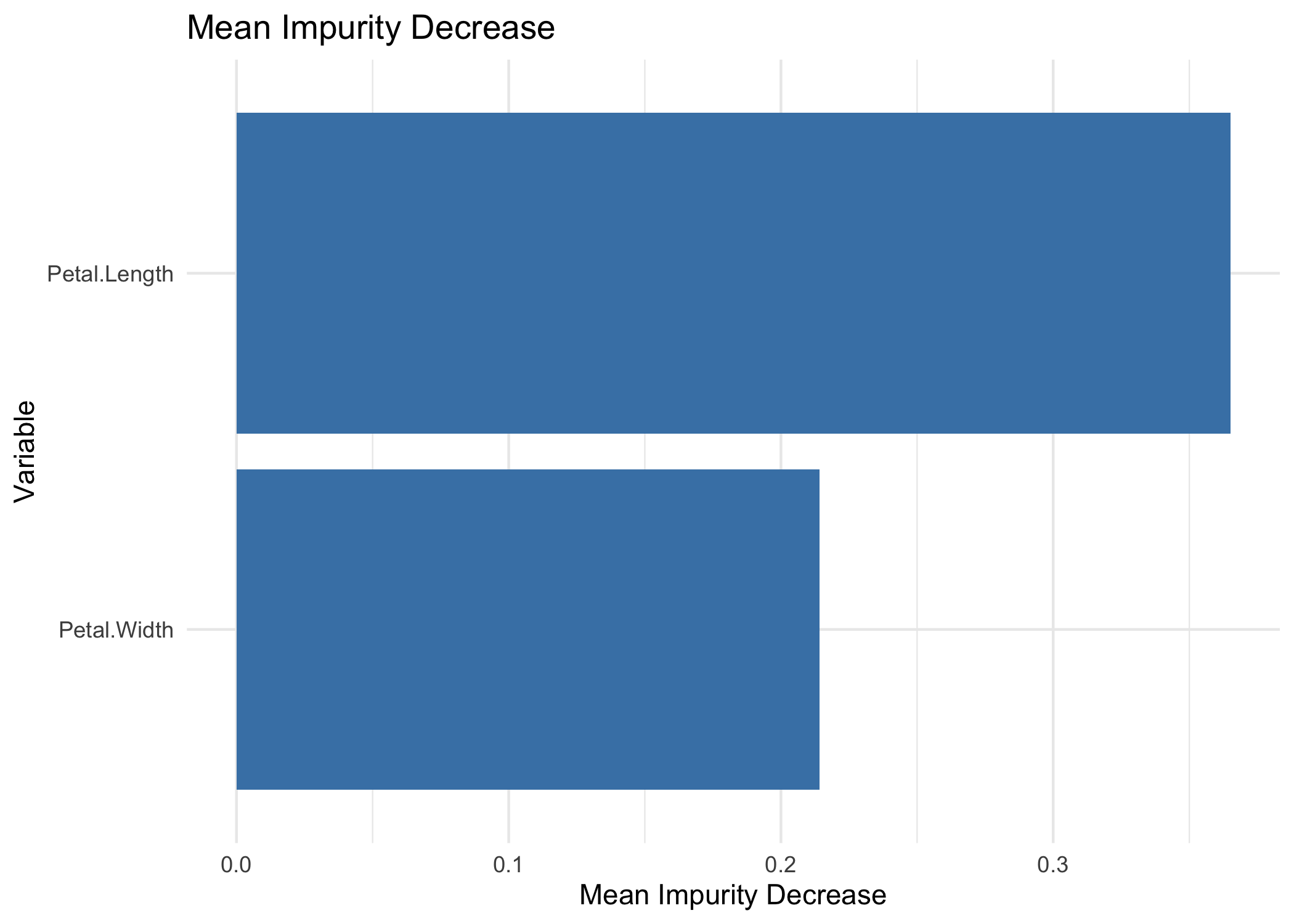
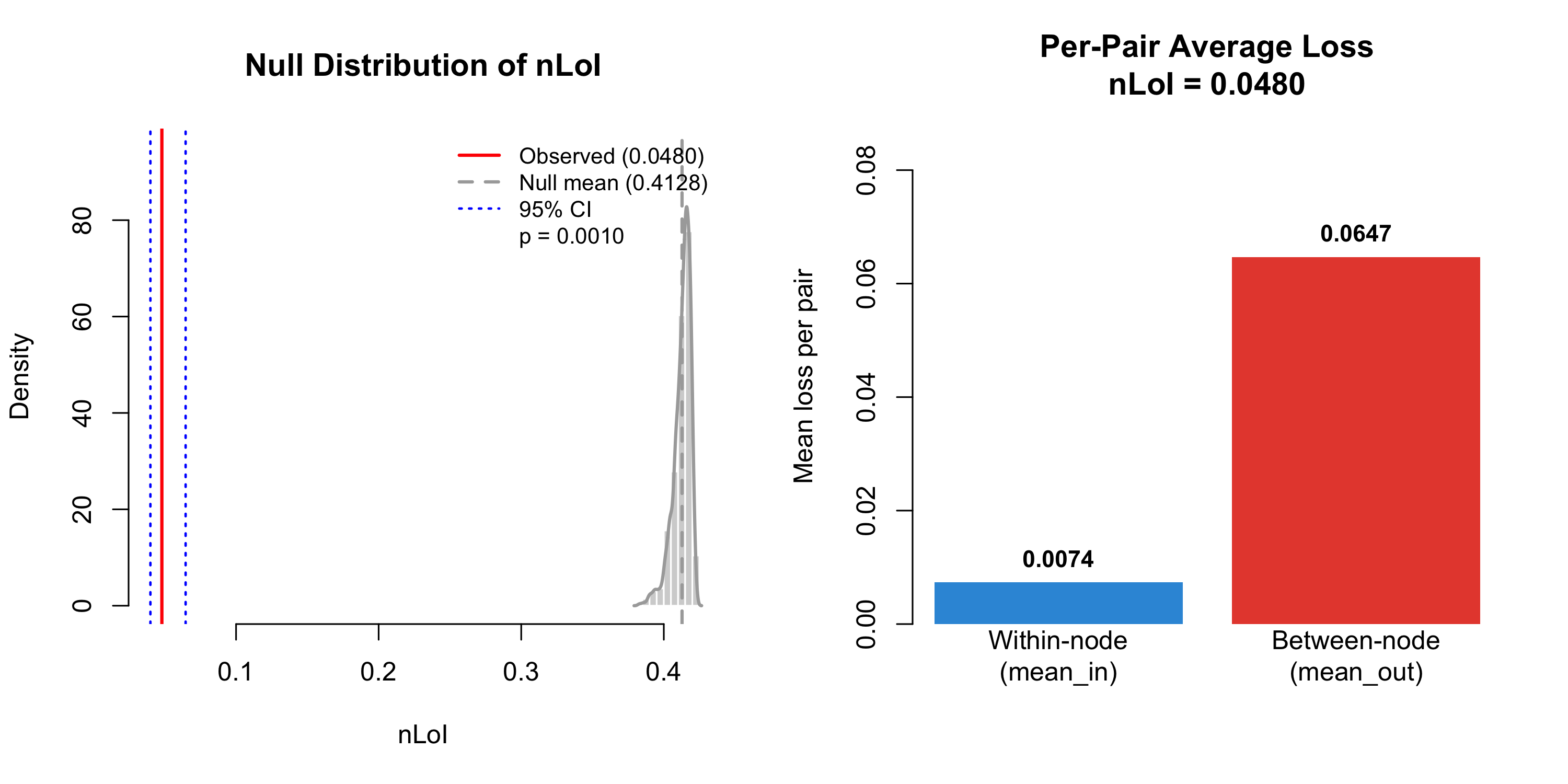
While vimp() summarises the overall contribution of each predictor, Local Observation Importance (loi()) attributes importance at the individual observation level — so you can explain why the model reached a specific conclusion for a specific case.
The local importance score for observation and variable is defined as:
where measures the change in the node's dissimilarity when variable j is excluded from the split at the node to which i belongs.
loi() — local importance scores per observationloi_perm() — permutation-based significanceplot() — visualise importance landscape
Install from CRAN and run the five-step workflow in a few minutes.